 |
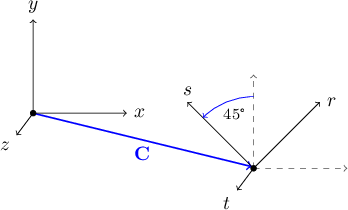
Figure 11.1: A reorientable object's $(r,s,t)$ axes start out identical to the camera's $(x,y,z)$ axes. |
All objects drawn by this ray tracing code must be instances of a class derived, directly or indirectly, from class SolidObject. Any such derived class, as discussed earlier, must implement virtual functions for translating and rotating the object. In the case of class Sphere, the Translate function is simple: it just moves the center of the sphere, and that center point is used by any code that calculates surface intersections, surface normal vectors, inclusion of a point within the sphere, etc. Rotation of the sphere is trivial in the extreme: rotating a sphere about its center has no effect on its appearance, so RotateX, RotateY, and RotateZ don't have to do anything.
However, the mathematical derivation of other shapes can be much more complicated, even if we were to ignore the need for translating and rotating them. Once translation and rotation are thrown into the mix, the resulting equations can become overwhelming and headache-inducing. For example, as I was figuring out how to draw a torus (a donut shape), the added complexity of arbitrarily moving and spinning the torus soon led me to think, "there has to be a better way to do this." I found myself wishing I could derive the intersection formulas for a shape located at a fixed position and orientation in space, and have some intermediate layer of code abstract away the problem of translation and rotation. I soon realized that I could do exactly that by converting the position and direction vectors passed into methods like AppendAllIntersections to another system of coordinates, doing all the math in that other coordinate system, and finally converting any intersections found the inverse way, back to the original coordinate system. In simple terms, the effect would be to rotate and translate the point of view of the camera in the opposite way we want the object to be translated and rotated. For example, if you wanted to photograph your living room rotated $15°$ to the right, it would be much easier to rotate your camera $15°$ to the left than to actually rotate your living room, and the resulting image would be the same (except your stuff would not be falling over, of course).
This concept is implemented by the class SolidObject_Reorientable, which derives from SolidObject. SolidObject_Reorientable acts as a translation layer between two coordinate systems: the $(x, y, z)$ coordinates we have been using all along, and a new set of coordinates $(r, s, t)$ that are fixed from the point of view of a reorientable object. I will refer to $(x, y, z)$ as camera space coordinates and $(r, s, t)$ as object space coordinates. Each reorientable object has its own object space $(r, s, t)$ coordinate system, independent of any other reorientable objects.
Class SolidObject_Reorientable introduces the following pure virtual methods that operate in object space, meaning they can be implemented with the assumption that the object resides at a fixed location and orientation with respect to an $(r, s, t)$ coordinate system:
    ObjectSpace_AppendAllIntersections
    ObjectSpace_Contains
These two methods are just like AppendAllIntersections and Contains as defined in class SolidObject, only they are passed vector parameters that have already been translated from camera coordinates to object coordinates. When an instance of a class derived from SolidObject_Reorientable is created, it starts out with $(r, s, t)$ axes identical to the camera's $(x, y, z)$ axes, as seen in Figure 11.1.
| |
|
If the object is then translated, the $(r, s, t)$ axes are shifted by the amounts specified by the translation vector, as show in Figure 11.2.
|
This is implemented by tracking the center of the object as usual, and shifting position vectors by subtracting the center position from the position of any $(x, y, z)$ location to get the (unrotated) $(r, s, t)$ coordinates.
If the object is rotated, the $(r, s, t)$ axes are rotated with respect to the $(x, y, z)$ axes. For example, RotateZ(45.0) applied to the example in Figure 11.2, where we had already translated the object, would cause the axes to look as shown in Figure 11.3.
| |
|
The $(r, s, t)$ axes have been rotated about the object's center, which is $(r,s,t)=(0,0,0)$ or $(x,y,z)=(C_x,C_y,C_z)$ by $45°$ counterclockwise parallel to the $z$ axis, looking into the $z$ axis, where $\mathbf{C} = (C_x, C_y, C_z)$ is the object's center as expressed in camera space.
How is rotation implemented in class SolidObject_Reorientable? First, let's take a look at that class's declaration in imager.h. You will find that the private section of this class contains two triplets of Vector-typed member variables, one triplet being rDir, sDir, and tDir, the other being xDir, yDir, and zDir. All of these vectors are unit vectors. The first three, rDir, sDir, and tDir, hold the direction in $(x, y, z)$ camera space that the $(r, s, t)$ object space axes point. Conversely, xDir, yDir, and zDir hold the directions in $(r, s, t)$ object space that the $(x, y, z)$ camera space axes point. As mentioned above, a newly-created reorientable object starts out with $(r, s, t)$ being identical to $(x, y, z)$, so these member variable vectors are initialized as follows by the SolidObject_Reorientable constructor:
    rDir=(1, 0, 0)    xDir=(1, 0, 0)
    sDir=(0, 1, 0)    yDir=(0, 1, 0)
    tDir=(0, 0, 1)    zDir=(0, 0, 1)
These are direction vectors, not position vectors, so they are not changed by the object being translated, but only when it is rotated. Translation affects only the center point position vector as reported by the protected member function SolidObject::Center. So the rotation problem breaks down into two questions:
The first question is easier to resolve if we use a trick from complex number arithmetic: a complex number is a pair of numbers, the first called the real part, the second called the imaginary part. They are often written as $a + ib$, with $a$ being the real part, $b$ being the imaginary part, and $i$ being the imaginary number $\sqrt{-1}$. If complex numbers are new to you, this idea probably seems bizarre and scary. But don't panic — for the purposes of this tutorial, there are only two things you need to know about complex numbers beyond basic algebra: first that $i^2 = -1$, and second that $a + ib$ can be thought of as just another way to write the two-dimensional vector $(a, b)$. If we are rotating an object parallel to the $z$ axis, we can pretend that all the object's points have their $x$ and $y$ components represented as complex numbers that get updated based on formulas I'm about to show you, and that their $z$ components remain unchanged. Likewise, rotation parallel to the $x$ axis involves $x$ components remaining unchanged while $y$ and $z$ are changed as if they were complex numbers of the form $y + iz$. The components must be kept in the order consistent with the right-hand rule, as discussed in the section on vector cross products. (See Table 11.1.)
| ||||||||||||
|
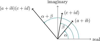
But how do complex numbers help us rotate two-dimensional vectors? I alluded to a trick, and here it is: when two complex numbers, say $a + ib$ and $c + id$ are multiplied, the product has the following relationship with the two complex numbers we started with:
Figure 11.4 illustrates these two rules.
| |
|
Multiplying complex numbers works using familiar rules of algebra:
\[ (a + ib)(c + id) = ac + ibc + iad + i^2bd \]
As noted above, $i^2 = -1$, so we can write the product as
\[ ac + ibd + iad - bd \]
Collecting the product terms into real and imaginary parts, we end up with
\[ (a + ib)(c + id) = (ac - bd) + i(bc + ad) \]
Or, if you prefer, the product can be written using two-dimensional vector notation to represent the complex numbers:
\[ (a,b)(c,d) = (ac-bd, bc+ad) \]
If we start with a two-dimensional vector $(c,d)$ and we want to rotate it by an angle $\theta$, all we need to do is to multiply it by the complex number $(a,b)$ that represents that angle, so long as the magnitude of $(a,b)$, or $\sqrt{a^2+b^2}$, is equal to 1. Here's how we calculate $(a,b)$:
\begin{align*} & a = \cos(\theta) \\ & b = \sin(\theta) \end{align*}
As we learned in Section 4.10, the point $(a,b) = (\cos(\theta),\sin(\theta))$ represents a point on a unit circle (a circle whose radius is one unit) at an angle $\theta$ measured counterclockwise from the positive horizontal axis. Because $\lvert (a,b) \rvert = \sqrt{a^2+b^2} = 1$, when we multiply $(a,b)$ by $(c,d)$, the product's magnitude will be the same as the magnitude of $(c,d)$. And, as we wanted from the start, the product's angle will be rotated by an angle $\theta$ with respect to $(c,d)$.
Depending on whether we are rotating parallel to the $x$, $y$, or $z$ axis — that is, whether RotateX, RotateY, or RotateZ is being called, we will apply the complex multiplication formula to the other two components: if rotating parallel to $x$, the $x$ component is not changed, but y and z are; if rotating parallel to $y$, the $y$ component is not changed, but $x$ and $z$ are modified, etc. In any case, all three of the unit vectors rDir, sDir, tDir are updated using the same formula (whichever formula is appropriate for that type of rotation) as shown in Table 11.2, where $(x, y, z)$ is the existing direction vector, and $(a, b) = (\cos(\theta), \sin(\theta))$.
| ||||||||||||
|
We are left with the related issue of how to update the unit vectors xDir, yDir, and zDir, each expressing in $(r, s, t)$ object coordinates how to convert vectors back into camera coordinates. This can be a confusing problem at first, because rotations are all parallel to the $x$, $y$, or $z$ axis, not $r$, $s$, $t$. If we were to rotate about $r$, $s$, or $t$, we could use the same complex number tricks, but that is not the case — an example of the difficulty is that RotateX never changes to $x$ component of rDir, sDir, or tDir, but it can change all of the components, $r$, $s$, and $t$, of xDir, yDir, and zDir.
But there is a surprisingly simple resolution of this confusing situation. Once we have calculated updated values for the unit vectors rDir, sDir, and tDir, we can arrange the three vectors, each having three components, in a 3-by-3 grid as shown in Table 11.3.
| |||||||||
|
Such a representation of three mutually perpendicular unit vectors has a name familiar to mathematicians and computer graphics experts: it is called a rotation matrix. Given these nine numbers, we want to calculate corresponding values for xDir, yDir, and zDir; these three unit vectors are known collectively as the inverse rotation matrix, since they will help us translate $(r, s, t)$ object space vectors back into $(x, y, z)$ camera space vectors. Remarkably, there is no need for any calculation effort at all; we merely need to rearrange the nine numbers from the original rotation matrix to obtain the inverse rotation matrix. The rows of the original matrix become the columns of the inverse matrix, and vice versa, as shown in Table 11.4.
| |||||||||
|
This rearrangement procedure is called transposition — we say that the inverse rotation matrix is the transpose of the original rotation matrix. So after we update the values of rDir, sDir, and tDir in RotateX, RotateY, or RotateZ, we just need to transpose the values into xDir, yDir, and zDir:
    xDir = Vector(rDir.x, sDir.x, tDir.x);
    yDir = Vector(rDir.y, sDir.y, tDir.y);
    zDir = Vector(rDir.z, sDir.z, tDir.z);
This block of code, needed by all three rotation methods, is encapsulated into the member function SolidObject_Reorientable::UpdateInverseRotation, which is located in imager.h. The code for RotateX, RotateY, and RotateZ is all located in reorient.cpp.
A point of clarification is helpful here. Although the vectors xDir, yDir, and zDir are object space vectors, and therefore contain $(r, s, t)$ components mathematically, they are implemented using the same C++ class Vector as is used for camera space vectors. This C++ class has members called x, y, and z, but we must understand that when class Vector is used for object space vectors, the members are to be interpreted as $(r, s, t)$ components. This implicit ambiguity eliminates otherwise needless duplication of code, avoiding a redundant version of class Vector (and its associated inline functions and operators) having members named r, s, and t.
At this point, we have completely resolved the problem of updating the six unit direction vectors as needed for calls to RotateX, RotateY, and RotateZ. Now we return to the second question: how do we use these vectors to translate back and forth between camera space and object space? The answer is: we use vector dot products. But we must take care to distinguish between vectors that represent directions and those that represent positions. Direction vectors are simpler, so we consider them first. Let $\mathbf{D} = (x, y, z)$ be a direction vector in camera space. We wish to find the object space direction vector $\mathbf{E} = (r, s, t)$ that points in the same direction. We already have computed the unit vectors rDir, sDir, and tDir, which specify $(x, y, z)$ values showing which way the $r$ axis, $s$ axis, and $t$ axis point. To calculate $r$, the $r$-component of the object space direction vector $\mathbf{E}$, we take advantage of the fact that the dot product of a direction vector with a unit vector tells us how much the direction vector extends in the direction of the unit vector. We take $\mathbf{D}\cdot$rDir as the value of $r$, thinking of that dot product as representing the "shadow" of $\mathbf{D}$ onto the $r$ axis.
The same analysis applies to $s$ and $t$, yielding the equations
\begin{align*} & r = \mathbf{D} \cdot \text{rDir} \\ & s = \mathbf{D} \cdot \text{sDir} \\ & t = \mathbf{D} \cdot \text{tDir} \end{align*}
If you look inside class SolidObject_Reorientable in the header file imager.h, you will find the following function that performs these calculations:
Vector ObjectDirFromCameraDir(const Vector& cameraDir) const
{
    return Vector(
        DotProduct(cameraDir, rDir),
        DotProduct(cameraDir, sDir),
        DotProduct(cameraDir, tDir)
    );
}
To compute the inverse, that is, a camera direction vector from an object direction vector, we use the function CameraDirFromObjectDir, which is almost identical to ObjectDirFromCameraDir, only it computes dot products with xDir, yDir, zDir instead of rDir, sDir, tDir.
Dealing with position vectors (that is, points) is only slightly more complicated than direction vectors. They require us to adjust for translations the object has experienced, based on the center position reported by the member function SolidObject::Center. Here are the corresponding functions for converting points from camera space to object space and back:
Vector ObjectPointFromCameraPoint(const Vector& cameraPoint) const
{
    return ObjectDirFromCameraDir(cameraPoint - Center());
}

Vector CameraPointFromObjectPoint(const Vector& objectPoint) const
{
    return Center() + CameraDirFromObjectDir(objectPoint);
}
Now that all the mathematical details of converting back and forth between camera space and vector space have been taken care of, it is fairly straightforward to implement SolidObject_Reorientable methods like AppendAllIntersections, shown here as it appears in reorient.cpp:
void SolidObject_Reorientable::AppendAllIntersections(
    const Vector& vantage,
    const Vector& direction,
    IntersectionList& intersectionList) const
{
    const Vector objectVantage = ObjectPointFromCameraPoint(vantage);
    const Vector objectRay     = ObjectDirFromCameraDir(direction);

    const size_t sizeBeforeAppend = intersectionList.size();

    ObjectSpace_AppendAllIntersections(
        objectVantage,
        objectRay,
        intersectionList
    );

    // Iterate only through the items we just appended,
    // skipping over anything that was already in the list
    // before this function was called.
    for (size_t index = sizeBeforeAppend;
         index < intersectionList.size();
         ++index)
    {
        Intersection& intersection = intersectionList[index];

        // Need to transform intersection back into camera space.
        intersection.point =
            CameraPointFromObjectPoint(intersection.point);

        intersection.surfaceNormal =
            CameraDirFromObjectDir(intersection.surfaceNormal);
    }
}
Note that this function translates parameters expressed in camera coordinates to object coordinates, calls ObjectSpace_AppendAllIntersections, and converts resulting object space vectors (intersection points and surface normal vectors) back into camera space, as the caller expects.
To illustrate how to use SolidObject_Reorientable as a base class, let's start with a very simple mathematical shape, the cuboid. A cuboid is just a rectangular box: it has six rectangular faces, three pairs of which are parallel and at right angles to the remaining pairs. The cuboid's length, width, and height may have any desired positive values.
We use $a$ to refer to half of the cuboid's width, $b$ for half of its length, and $c$ for half its height, so its dimensions are $2a$ by $2b$ by $2c$. This approach simplifies the math. For example, the left face is at $r = -a$, the right face is at $r = +a$, etc. Note that using object space coordinates $r$, $s$, and $t$ allows us to think of the cuboid as locked in place, with the $(r,s,t)$ origin always at the center of the cuboid and the three axes always orthogonal with the cuboid's faces.
The class Cuboid is declared in the header file imager.h as follows:
// A "box" with rectangular faces, all of which are mutually perpendicular.
class Cuboid: public SolidObject_Reorientable
{
public:
    Cuboid(double _a, double _b, double _c, Color _color)
        : SolidObject_Reorientable()
        , color(_color)
        , a(_a)
        , b(_b)
        , c(_c)
    {
    }

    Cuboid(double _a, double _b, double _c,
           Color _color, const Vector& _center)
        : SolidObject_Reorientable(_center)
        , color(_color)
        , a(_a)
        , b(_b)
        , c(_c)
    {
    }

protected:
    virtual size_t ObjectSpace_AppendAllIntersections(
        const Vector& vantage,
        const Vector& direction,
        IntersectionList& intersectionList) const;

    virtual bool ObjectSpace_Contains(const Vector& point) const
    {
        return
            (fabs(point.x) <= a + EPSILON) &&
            (fabs(point.y) <= b + EPSILON) &&
            (fabs(point.z) <= c + EPSILON);
    }

private:
    const Color     color;
    const double    a;      // half of the width
    const double    b;      // half of the length
    const double    c;      // half of the height
};
The Cuboid class is a good example of the minimal steps needed to create a reorientable solid class:
The ObjectSpace_Contains function is very simple thanks to fixed object space coordinates: a point is inside the cuboid if $-a \le r \le +a$, $-b \le s \le +b$, and $-c \le t \le +c$. Because the function's point parameter is of type Vector, the C++ code requires us to type point.x, point.y, and point.z, but we understand these to refer to the point's $r$, $s$, and $t$ components. Also, to provide tolerance for floating point rounding errors, we widen the ranges of inclusion by the small amount EPSILON. This method will be used in ObjectSpace_AppendAllIntersections, and using EPSILON like this helps ensure that we correctly include intersection points in the result. (The extra tolerance will also be necessary to use Cuboid as part of a set operation, a topic that is covered in a later chapter.) Using the standard library's absolute value function fabs, we therefore express $-a \le r \le +a$ as
fabs(point.x) <= a + EPSILON
and so on.
Coding the method Cuboid::ObjectSpace_AppendAllIntersections
requires the same kind of mathematical approach we used in Sphere::AppendAllIntersections:
| ||||||||||||||
|
\begin{align*} \mathbf{P} & = \mathbf{D} + u \mathbf{E} \\ & = (D_r, D_s, D_t) + u(E_r, E_s, E_t) \end{align*}
For the point $\mathbf{P}$ to be on the left face, its $r$ component must be equal to $-a$, so:\[ D_r + u E_r = -a \]
Solving for the parameter $u$, we find\[ u = \frac{-a - D_r}{E_r}, \quad E_r \ne 0, \quad u > 0. \]
Substituting $u$ back into the parametric ray equation, we find the values of the $s$ and $t$ components of $\mathbf{P}$, completely determining the point $\mathbf{P}$:\[ \mathbf{P} = (-a, D_s + u E_s, D_t + u E_t) \]
If we find that $s = D_s + u E_s$ is in the range $-b$...$+b$ and that $t = D_t + u E_t$ is in the range $-c$...$+c$ (that is, that ObjectSpace_Contains(P) returns true), we know that the intersection point is genuinely on the cuboid's left face. As always, we have to check that $u >$ EPSILON, ensuring that the intersection point is significantly in the intended direction $\mathbf{E}$ from the vantage point $\mathbf{D}$, not at $\mathbf{D}$ or in the opposite direction $-\mathbf{E}$.The code for the remaining five faces is very similar, as you can see by looking at cuboid.cpp.
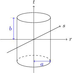
Let's take a look at another reorientable solid: the Cylinder class. A cylinder is like an idealized soup can, consisting of three surfaces: a curved lateral tube and two circular discs, one on the top and another on the bottom. This time I will cover the mathematical solution for finding intersections between a ray and a cylinder and for the surface normal vector at an intersection, but I will omit discussion of the coding details, as they are very similar to what we already covered in class Cuboid.
| |
|
The cylinder is aligned along the $t$ axis, with its top disc located at $t = +b$ and its bottom disc at $t = -b$. The discs and the lateral tube have a common radius $a$. These three surfaces have the equations and constraints as shown in Table 11.6.
| ||||||||||||
|
The tube equation derives from taking any cross-section of the cylinder parallel to the $rs$ plane and between the top and bottom discs. You would be cutting through a perfect circle: the set of points in the cross-sectional plane that measure $a$ units from the $t$ axis. The value of $t$ where you cut is irrelevant — you simply have the formula for a circle of radius $a$ on the $rs$ plane, or $r^2 + s^2 = a^2$.
As usual, we find the simultaneous solution of the parametric ray equation with each of the surface equations, yielding potential intersection points for the corresponding surfaces. Each potential intersection is valid only if it satisfies the constraint for that surface.
The equations for the discs are simpler than the tube equation, so we start with them. We can write both equations with a single expression:
\[ t = \pm b \]
Then we combine the disc surface equations with the parametric ray equation:
\begin{align*} \mathbf{P} & = \mathbf{D} + u \mathbf{E} \\ (r,s,t) & = (D_r, D_s, D_t) + u(E_r, E_s, E_t) \\ (r,s,t) & = (D_r + u E_r, D_s + u E_s, D_t + u E_t) \end{align*}
In order for a point $\mathbf{P}$ on the ray to be located on one of the cylinder's two discs, the $t$ component must be either $-b$ or $+b$:
\[ D_t + u E_t = \pm b \]
Solving for $u$, we find
\[ u = \frac{\pm b - D_t}{E_t}, \quad E_t \ne 0 \]
Assuming $u > 0$, the potential intersection points for the discs are
\[ \left( D_r + \left( \frac{\pm b - D_t}{E_t} \right) E_r \, , \; D_s + \left( \frac{\pm b - D_t}{E_t} \right) E_s \, , \; \pm b \right) \]
Letting $r = D_r + \left( \frac{\pm b - D_t}{E_t} \right) E_r$ and $s = D_s + \left( \frac{\pm b - D_t}{E_t} \right) E_s$, we check the constraint $r^2 + s^2 \le a^2$ to see if each value of $\mathbf{P}$ is within the bounds of the disc. If so, the surface normal vector is $(0, 0, 1)$ for any point on the top disc, or $(0, 0, -1)$ for any point on the bottom disc — a unit vector perpendicular to the disc and outward from the cylinder in either case.
We turn our attention now to the problem of finding intersections of a ray with the lateral tube. Just as in the case of a sphere, a ray may intersect a tube in two places, so we should expect to end up having a quadratic equation. We find that the simultaneous solution of the parametric ray equation and the surface equation for the tube gives us exactly that:
\[ \begin{cases} & (r,s,t) = (D_r + u E_r, D_s + u E_s, D_t + u E_t) \\ & r^2 + s^2 = a^2 \end{cases} \]
We substitute the values $r = D_r + u E_r$ and $s = D_s + u E_s$ from the ray equation into the tube equation:
\[ (D_r + u E_r)^2 + (D_s + u E_s)^2 = a^2 \]
The only unknown quantity in this equation is $u$, and we wish to solve for it in terms of the other quantities. The algebra proceeds as follows:
\[ (D_r^2 + 2 D_r E_r u + E_r^2 u^2) + (D_s^2 + 2 D_s E_s u + E_s^2 u^2) = a^2 \]
\[ (E_r^2 + E_s^2)u^2 + 2(D_r E_r + D_s E_s)u + (D_r^2 + D_s^2 - a^2) = 0 \]
Letting
\[ \begin{cases} & A = E_r^2 + E_s^2 \\ & B = 2(D_r E_r + D_s E_s) \\ & C = D_r^2 + D_s^2 - a^2 \end{cases} \]
we have a quadratic equation in standard form:
\[ A u^2 + B u + C = 0 \]
As in the case of the sphere, we try to find real and positive values of $u$ via
\[ u = \frac{-B \pm \sqrt{B^2 - 4 A C}}{2A} \]
If $B^2 - 4 A C < 0$, we give up immediately. The imaginary result of taking the square root of a negative number is our signal that the ray does not intersect with an infinitely long tube of radius $r$ aligned along the $t$ axis, let alone the finite cylinder. But if $B^2 - 4 A C \ge 0$, we use the formula above to find two real values for $u$. As before, there are two extra hurdles to confirm that the point $\mathbf{P}$ is on the tube: $u$ must be greater than 0 (or EPSILON in the C++ code, to avoid rounding error problems) and $t = D_t + u E_t$ must be in the range $-b \le t \le +b$ (or $\lvert t \rvert \le b +$ EPSILON, again to avoid roundoff error problems).
When we do confirm that an intersection point lies on the tube's surface, we need to calculate the surface normal unit vector at that point. To be perpendicular to the tube's surface, the normal vector must point directly away from the center of the tube, and be parallel with the top and bottom discs.
The normal vector $\mathbf{\hat{n}}$ must lie in a plane that includes the intersection point $\mathbf{P}$ and that is parallel to the $rs$ plane. As such, $\mathbf{\hat{n}}$ is perpendicular to the $t$ axis, so its $t$ component is zero. If we let $\mathbf{Q}$ be the point along the $t$ axis that is closest to the intersection point $\mathbf{P} = (P_x, P_y, P_z)$, we can see that $\mathbf{Q} = (0, 0, P_z)$. The vector difference $\mathbf{P} - \mathbf{Q} = (P_x, P_y, 0)$ points in the same direction as $\mathbf{\hat{n}}$, but has magnitude $\lvert \mathbf{P} - \mathbf{Q} \rvert = a$, where $a$ is the radius of the cylinder. To convert to a unit vector, we must divide the vector difference by its magnitude:
\[ \mathbf{\hat{n}} = \frac{\mathbf{P} - \mathbf{Q}}{a} = \left(\frac{P_x}{a}, \frac{P_y}{a}, 0 \right) \]
We now have a complete mathematical solution for rendering a ray-traced image of a cylinder. The C++ implementation details are all available in the declaration for class Cylinder in imager.h and the function bodies in cylinder.cpp.